vector data
1. Import geometry data
[1]:
# !pip install h3-toolkit, geopandas, polars, psycopg2-binary, sqlalchemy, geoalchemy2, connectorx
[2]:
import os

import geopandas as gpd
import polars as pl
from dotenv import load_dotenv
from sqlalchemy import create_engine

load_dotenv()
URI = os.getenv("POSTGRES")
1.1. Use geopandas to fetch vector data from Postgis (slowly)
CSL researcher only
[3]:
sql = """
with boundary as (
    select 代碼, geometry
    from geometry.boundary_smallest
    where 縣市代碼 = %(city_code)s
)
select aps.*, boundary.geometry as geometry
from geometry.af_ppl_stats as aps
join boundary
on aps.codebase = boundary.代碼
"""

engine = create_engine(URI)
with engine.connect() as conn:
    gdf = gpd.read_postgis(
        sql,
        con=conn.connection,
        geom_col='geometry',
        params={'city_code': '63000'} # 台北市
    )
/Users/syuanbo/Documents/GitHub/H3-ToolKits/.venv/lib/python3.12/site-packages/geopandas/io/sql.py:185: UserWarning: pandas only supports SQLAlchemy connectable (engine/connection) or database string URI or sqlite3 DBAPI2 connection. Other DBAPI2 objects are not tested. Please consider using SQLAlchemy.
  df = pd.read_sql(
/Users/syuanbo/Documents/GitHub/H3-ToolKits/.venv/lib/python3.12/site-packages/geopandas/io/sql.py:473: UserWarning: pandas only supports SQLAlchemy connectable (engine/connection) or database string URI or sqlite3 DBAPI2 connection. Other DBAPI2 objects are not tested. Please consider using SQLAlchemy.
  return pd.read_sql(spatial_ref_sys_sql, con)
[4]:
gdf.head()
[4]:
| codebase | city | h_cnt | p_cnt | m_cnt | f_cnt | info_time | geometry | |
|---|---|---|---|---|---|---|---|---|
| 0 | A6301-0097-00 | 臺北市 | 40 | 121 | 53 | 68 | 2023-12-01 00:00:00+00:00 | MULTIPOLYGON (((121.54425 25.06221, 121.54466 ... |
| 1 | A6303-0422-00 | 臺北市 | 146 | 376 | 165 | 211 | 2023-12-01 00:00:00+00:00 | MULTIPOLYGON (((121.55701 25.03439, 121.5575 2... |
| 2 | A6303-1146-00 | 臺北市 | 93 | 229 | 110 | 119 | 2023-12-01 00:00:00+00:00 | MULTIPOLYGON (((121.55202 25.02088, 121.55205 ... |
| 3 | A6311-0203-00 | 臺北市 | 58 | 159 | 80 | 79 | 2023-12-01 00:00:00+00:00 | MULTIPOLYGON (((121.5243 25.11859, 121.52431 2... |
| 4 | A6308-0588-00 | 臺北市 | 112 | 299 | 142 | 157 | 2023-12-01 00:00:00+00:00 | MULTIPOLYGON (((121.57742 24.99215, 121.57746 ... |
1.2. Use polars+connectorx to fetch vector data from Postgis (faster, recommended)
CSL researcher only
[5]:
city_code = 63000

sql = f"""
with boundary as (
    select 代碼, geometry
    from geometry.boundary_smallest
    where 縣市代碼 = {city_code}
)
select aps.*, ST_AsBinary(boundary.geometry) as geometry_wkb
from geometry.af_ppl_stats as aps
join boundary
on aps.codebase = boundary.代碼
"""

pdf = pl.read_database_uri(sql, URI, engine="connectorx")
pdf.head()
[5]:
| codebase | city | h_cnt | p_cnt | m_cnt | f_cnt | info_time | geometry_wkb |
|---|---|---|---|---|---|---|---|
| str | str | i64 | i64 | i64 | i64 | datetime[ns, UTC] | binary |
| "A6303-0422-00" | "臺北市" | 146 | 376 | 165 | 211 | 2023-12-01 00:00:00 UTC | b"\x01\x06\x00\x00\x00\x01\x00\x00\x00\x01\x03\x00\x00\x00\x01\x00\x00\x00\x09\x00\x00\x00\x14\x9c\xfc\x15\xa6c^@\xa5\xa9\xb8\x9a\xcd\x089@v\xd7\xe3&\xaec^@\x09\xbfMB\xcd\x089@\xef\xe7\x99\x1c\xaec"... |
| "A6303-1146-00" | "臺北市" | 93 | 229 | 110 | 119 | 2023-12-01 00:00:00 UTC | b"\x01\x06\x00\x00\x00\x01\x00\x00\x00\x01\x03\x00\x00\x00\x01\x00\x00\x00\x0b\x00\x00\x006W\xca>Tc^@\x9a\xdb\x15GX\x059@\x0d\x06\x09\xdeTc^@&\x09\x07pV\x059@x\xcd\x94\x9cVc"... |
| "A6311-0203-00" | "臺北市" | 58 | 159 | 80 | 79 | 2023-12-01 00:00:00 UTC | b"\x01\x06\x00\x00\x00\x01\x00\x00\x00\x01\x03\x00\x00\x00\x01\x00\x00\x00\x0b\x00\x00\x00\:83\x8ea^@\xee\x9a\x1a\xc5[\x1e9@\xe3'-:\x8ea^@\xc0n2\xc0[\x1e9@Jz\xd9\xf1\x92a"... |
| "A6308-0588-00" | "臺北市" | 112 | 299 | 142 | 157 | 2023-12-01 00:00:00 UTC | b"\x01\x06\x00\x00\x00\x01\x00\x00\x00\x01\x03\x00\x00\x00\x01\x00\x00\x00\x1d\x00\x00\x00\V,o\xf4d^@H\xa8\x11\xcc\xfd\xfd8@qV\x9b\x09\xf5d^@\xc3\x93j\x8d\xf2\xfd8@O\x94G\xf6\xf4d"... |
| "A6310-1111-00" | "臺北市" | 0 | 0 | 0 | 0 | 2023-12-01 00:00:00 UTC | b"\x01\x06\x00\x00\x00\x01\x00\x00\x00\x01\x03\x00\x00\x00\x01\x00\x00\x00"\x00\x00\x00Q\x91;\xf2\x9ce^@\x99\xc8\x19\xd8\xec\x109@-\xcf\xdd\xb4\xa3e^@!\xcfp\x09\xe1\x109@m%\xfa3\xa5e"... |
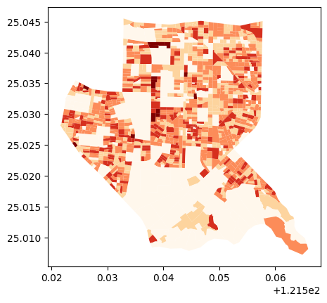
1.3. Use geopandas to read geometry file
[6]:
data = gpd.read_file('data/test_geom.geojson')
data.plot(column='p_cnt',
               cmap='OrRd',         # 使用顏色映射
               scheme='naturalbreaks',  # 自然斷點分類
               k=5,
               legend=False
)
[6]:
<Axes: >
2. Geometry to h3
The H3Toolkit is a chainable class that can convert geometry data to h3 index.
Step1: use
set_aggregation_strategy()to set the target column and the aggregation method in the dict{ column_name : aggregation_function() }.Step2: use
process_from_vector()to set the data and the h3 resolution, this function will convert the geometry to h3 index in the designated resolution and process the column(s) with the aggregation method you set.Step3: use
get_result()to get the result. default is a polars dataframe with the h3 index and the aggregated column(s), if you want the actual geometry, you can setreturn_geometry=Trueto get the geometry column, and the return type will be the geopandas dataframe.
NOTE: this function always use the centroid of the h3 hexagon to extract the data from actual geometry object, so the result may loss some information if you choose the inproper resolution. If missing data exists, the warnging will be raised. you should choose the proper resolution to avoid this situation, ie from resolution 7 to 10. if you want the lower resolution, you can chain the result from process_from_vector() to process_from_h3() to get the lower resolution h3 index without
lossing any information.
must to use get_result() to get the result, otherwise return will be the H3Toolkit object.
[7]:
from h3_toolkit import H3Toolkit
from h3_toolkit.aggregation import EqualSplit

toolkit = H3Toolkit()

result = (
    toolkit
    .set_aggregation_strategy(
        {
            'p_cnt' : EqualSplit(agg_col='codebase'),
        }
    )
    .process_from_vector(data, resolution=12, geometry_col='geometry')
)

output_df = result.get_result()

output_df.head()
[7]:
| hex_id | p_cnt |
|---|---|
| str | f64 |
| "8c4ba0a412a01ff" | 14.208333 |
| "8c4ba0a412a05ff" | 14.208333 |
| "8c4ba0a412a07ff" | 14.208333 |
| "8c4ba0a412a09ff" | 14.208333 |
| "8c4ba0a412a0bff" | 14.208333 |
set return_geometry=True to get the geometry column in the result.
[8]:
output_gdf = result.get_result(return_geometry=True, fill_null_value=0)
output_gdf.head()
[8]:
| hex_id | p_cnt | geometry | |
|---|---|---|---|
| 0 | 8c4ba0a412a01ff | 14.208333 | POLYGON ((121.54706 25.04487, 121.54705 25.044... |
| 1 | 8c4ba0a412a05ff | 14.208333 | POLYGON ((121.54695 25.04474, 121.54694 25.044... |
| 2 | 8c4ba0a412a07ff | 14.208333 | POLYGON ((121.54713 25.04473, 121.54711 25.044... |
| 3 | 8c4ba0a412a09ff | 14.208333 | POLYGON ((121.547 25.04501, 121.54698 25.04492... |
| 4 | 8c4ba0a412a0bff | 14.208333 | POLYGON ((121.54717 25.045, 121.54716 25.04491... |
3. Scale current h3 resolution to the target resolution
scale up the h3 index to the target resolution, the process_from_h3() function will do this job.
NOTE: The source_resolution must be greater than the target_resolution, otherwise the result will be wrong.
[9]:
from h3_toolkit import H3Toolkit
from h3_toolkit.aggregation import Sum

toolkit = H3Toolkit()

result = (
    toolkit
    .set_aggregation_strategy(
        {
            'p_cnt' : Sum(),
        }
    )
    .process_from_h3(
        output_df,
        source_resolution=12,
        target_resolution=10,
        h3_col='hex_id'
    )
)

output_df_10 = result.get_result(fill_null_value=0)
output_df_10.head()
[9]:
| hex_id | p_cnt |
|---|---|
| str | f64 |
| "8a4ba0a5d18ffff" | 23.007257 |
| "8a4ba0a43c4ffff" | 603.692149 |
| "8a4ba0a4e99ffff" | 199.093091 |
| "8a4ba0a5d19ffff" | 11.574834 |
| "8a4ba0a5db57fff" | 485.178707 |
Now, you are successfully scale up the data from resolution 12 to 10.
The benefit of H3Toolkit is that you can chain all the functions together, it’s much simple and maintainable. and make the process logic more clear!
[10]:
toolkit = H3Toolkit()

result = (
    toolkit
    .set_aggregation_strategy(
        {
            ('p_cnt', 'h_cnt') : EqualSplit(agg_col='codebase'),
        }
    )
    .process_from_vector(data, resolution=12, geometry_col='geometry')
    .set_aggregation_strategy(
        {
            ('p_cnt', 'h_cnt') : Sum(),
        }
    )
    .process_from_h3(
        source_resolution=12,
        target_resolution=10,
        h3_col='hex_id'
    )
    .get_result()
)

result.head()
[10]:
| hex_id | p_cnt | h_cnt |
|---|---|---|
| str | f64 | f64 |
| "8a4ba0a4e847fff" | 595.238028 | 248.036192 |
| "8a4ba0a5d30ffff" | 2.853159 | 1.233115 |
| "8a4ba0a4301ffff" | 868.195243 | 351.344298 |
| "8a4ba0a4e557fff" | 587.340822 | 231.649744 |
| "8a4ba0a5d8f7fff" | 9.990734 | 3.819245 |
4. Visualization
Use the show_h3() function from h3_toolkit.visualization module to visualize the h3 data interactively with pydeck.
Supported classifiers (from mapclassify): NaturalBreaks, Quantiles, EqualInterval, Jenks, and more. Supported colormaps (from matplotlib): Oranges, viridis, RdYlGn, Blues, Greens, and many others.
[ ]:
from h3_toolkit.visualization import show_h3

# Visualize with default classifier (NaturalBreaks) and colormap (Oranges)
show_h3(output_df, 'p_cnt')
[ ]:
# Visualize resolution 12 data with default NaturalBreaks classifier
toolkit.show(target_col='p_cnt')
Due to performance limitations when rendering large H3 datasets on the web, here’s a screenshot example of the visualization. For an interactive map, you can clone the notebook and run it locally in your environment

[ ]:
# Visualize resolution 10 data with Quantiles classifier
show_h3(output_df_10, 'p_cnt', classifier='Quantiles', k=5)
Due to performance limitations when rendering large H3 datasets on the web, here’s a screenshot example of the visualization. For an interactive map, you can clone the notebook and run it locally in your environment

It’s not recommended using pydeck or kepler.gl to visualize the h3 data if the data is too large, because the h3 data is too dense to visualize, it will be very slow and may crash.
The better way to visual large dataset is using lonboard, but this package is not support the h3 data yet, so you should convert the h3 data to the geometry data before visualizing it.
[14]:
## TODO: Use case of lonborad
5. Customize the aggregation function
We provided some popular aggregation methods for doing the aggregation, read the h3_toolkit.aggregation class to get more information.
But you can also custom your specific aggregation function by yourself, just define a function that inherit from the AggregationStrategy class and implement the apply() function.
[15]:
from h3_toolkit import H3Toolkit
from h3_toolkit.aggregation import AggregationStrategy


class NewAggregationStrategy(AggregationStrategy):
    """
    Make sure to inherit from AggregationStrategy and implement the apply method
    with data and target_cols attributes.
    """
    def __init__(self, new_var):
        """
        If you want to pass some parameters to the strategy, you can do it here.
        """
        self.new_var = new_var


    def apply(data:pl.DataFrame, target_cols:list[str]) -> pl.DataFrame:
        """
        If you are not familiar with polars, you can use pandas instead.
        just make sure to convert the type to polars dataframe before returning it.
        >>> data = data.to_pandas()
        >>> ...
        >>> ...
        >>> ...
        >>> return pl.from_pandas(data)
        """
        pass


toolkit = H3Toolkit()
toolkit.set_aggregation_strategy(
    {
        ('col_name', '...') : NewAggregationStrategy(new_var='...'),
    }
)
[15]:
<h3_toolkit.core.H3Toolkit at 0x14396b2c0>