raster data

import os

import geopandas as gpd
import polars as pl
import psycopg2
from dotenv import load_dotenv

load_dotenv()
URI = os.getenv("POSTGRES")

1. Fetch raster data

1.1. fetch from PostGIS

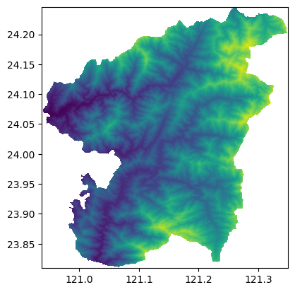
The example here is the DTM raster data from Renai Nantou, Taiwan. The data is stored in a PostGIS database. We will fetch the data and display it using the rasterio library.

from rasterio.io import MemoryFile
from rasterio.plot import show


with psycopg2.connect(URI) as conn:
    with conn.cursor() as cur:
        cur.execute('''
        SET postgis.gdal_enabled_drivers TO 'GTiff';

        WITH boundary AS (
        SELECT geometry as geom
        FROM geometry.boundary_town
        WHERE city_name = '南投縣' and town_name = '仁愛鄉'
        )
        SELECT ST_AsGDALRaster(
            ST_Union(ST_Clip(rast, geom)), 'GTiff'
            ) AS clipped_raster
        FROM geometry.nature_dtm, boundary
        WHERE ST_Intersects(rast, geom)
        ''')

        for row in cur:
            rast = row[0].tobytes()
            with MemoryFile(rast).open() as dataset:
                data_array = dataset.read()
                transform = dataset.transform
                nodata_value = dataset.nodata
                show(dataset)

1.2. Use rasterio to read raster data

NOTE: Before processing raster data to h3, you have to check the crs of the raster data. If the crs is not EPSG:4326, you have to reproject the raster data to EPSG:4326.

import rasterio as rio

with rio.open('data/test_raster.tif') as src:
    data = src.read()
    transform = src.transform
    nodata = src.nodata
    show(src)

2. Convert raster to h3

use process_from_raster() function to convert raster to h3, don’t need to set_aggregation_strategy, because the process_from_raster() can only accept one band at the time (2D array).

from h3_toolkit import H3Toolkit

toolkit = H3Toolkit()

result = (
    toolkit
    .process_from_raster(
        data = data_array[0],
        transform = transform,
        resolution = 12,
        nodata_value= int(nodata_value)
    )
)

output_12 = result.get_result()
output_12.head()

shape: (5, 2)

hex_id	value
str	i16
"8c4ba068a01b5ff"	3114
"8c4ba068a0517ff"	3114
"8c4ba068a0a2dff"	3114
"8c4ba068a0b53ff"	3114
"8c4ba068a1831ff"	3114

3. Scale current h3 resolution to the target resolution

from h3_toolkit.aggregation import Mean

toolkit = H3Toolkit()

result = (
    toolkit
    .set_aggregation_strategy(
        {
            'value': Mean()
        }
    )
    .process_from_h3(
        data = output_12,
        source_resolution = 12,
        target_resolution= 9,
        h3_col='hex_id'
    )
)

output_9 = result.get_result()
output_9.head()

shape: (5, 2)

hex_id	value
str	f64
"894ba2af297ffff"	1290.469388
"894ba2aeab7ffff"	1050.22449
"894ba2a6663ffff"	918.422741
"894ba068647ffff"	1881.798834
"894ba2a5647ffff"	701.043732

4. Visualization

import mapclassify as mc
import pandas as pd
import pydeck as pdk
from matplotlib import colormaps

INITIAL_VIEW_STATE = {
    'latitude':24.032518695904923,
    'longitude':121.15366859978752,
    'zoom':9.5,
    'max_zoom':13,
    'pitch':0,
    'bearing':0
}

def _set_color(
    data:pl.DataFrame | gpd.GeoDataFrame,
    target_col:str,
) -> pd.DataFrame | gpd.GeoDataFrame:
    """set color column for data based on target_col
    """

    # change this classifier to fit your data
    classifier = mc.NaturalBreaks(data[target_col], k=5)
    cmap = colormaps.get_cmap('Greens')

    if isinstance(data, pl.DataFrame):
        data = data.to_pandas()
    data['interval'] = classifier.find_bin(data[target_col])
    data['color'] = data['interval'].apply(lambda x: cmap(x / data['interval'].max()))
    data['color'] = data['color'].apply(lambda c: [int(255 * i) for i in c[:3]] + [255])
    data = data.drop(columns='interval')

    return data


def show_h3(
    data:pl.DataFrame,
    target_col:str,
    h3_col='hex_id'
):
    """show h3 hexagon layer
    """

    data = data.clone()
    data = _set_color(data, target_col)
    data = data.to_dict(orient='records')

    layer_h3 = pdk.Layer(
        'H3HexagonLayer',
        data,
        get_fill_color='color',
        # get_line_color=[255, 255, 255],
        # get_elevation='p_cnt',
        get_hexagon=h3_col,
        pickable=True,
        opacity=0.4,
        stroked=False,
        filled=True,
        extruded=False,
    )

    r = pdk.Deck(
        layers=[layer_h3],
        initial_view_state=pdk.ViewState(**INITIAL_VIEW_STATE),
        tooltip={"text": f"{target_col}: {{{target_col}}}"}
    )
    return r

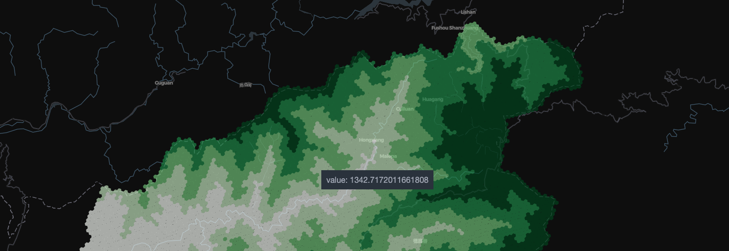
show_h3(output_9, 'value')

Due to performance limitations when rendering large H3 datasets on the web, here’s a screenshot example of the visualization. For an interactive map, you can clone the notebook and run it locally in your environment